An academic is expected to be a jack of many trades – handling research, teaching, mentorship, administration, committee work, reviewing, grant-writing, and editorial duties. Science communication is increasingly being added to that list as well. Outreach, public engagement and science communication are all terms thrown around (e.g. the 'Broader Impacts' section of many NSF grants, for example, includes the possibility "Broaden dissemination to enhance scientific and technological understanding"). Sometimes this can include communication between academics (conferences, seminars, blogs like this one) but often it is meant to include communication with the general public. Statistics about low science literacy at least partially motivate this. For example, “Between 29% and 57% of Americans responded correctly to various questions measuring the concepts of scientific experiment and controlling variables. Only 12% of Americans responded correctly to all the questions on this topic, and nearly 20% did not respond correctly to any of them”. (http://www.nsf.gov/statistics/seind14/index.cfm/chapter-7/c7s2.htm).
Clearly improving scientific communication is a worthy goal. But at times it feels like it is a token addition to an application, one that is outsourced to scientists without providing the necessary resources or training. . This is a problem because if we truly value scientific communication, the focus should be on doing it in a thoughtful manner, rather than as an afterthought. I say this because firstly because communicating complex ideas, some of which may require specialized terms and background knowledge, is difficult. The IPCC summaries, meant to be accessible to lay readers were recently reported to be incredibly inaccessible to the average reader (and getting worse over time!). Their Flesch reading ease scores were lower than those of Einstein’s seminal papers, and certainly far lower than most popular science magazines. Expert academics, already stretched between many skills, may not always be the best communicators of their own work.
Secondly, even when done well, it should be recognized that the audience for much science communication is a minority of all media consumers – the ‘science attentive’ or ‘science enthusiast’ portion of the public. Popular approaches to communication are often preaching to the choir. And even within this group, there are topics that naturally draw more interest or are innately more accessible. Your stochastic models will inherently be more difficult to excite your grandmother about than your research on the extinction of a charismatic furry animal. Not every topic is going to be of interest to a general audience, or even a science-inclined audience, and that should be okay.
So what should our science communication goals be, as scientists and as a society? There is entire literature on this topic (the science of science communication, so to speak), and it provides insight into what works and what is needed. However, “....despite notable new directions, many communication efforts continue to be based on ad-hoc, intuition-driven approaches, paying little attention to several decades of interdisciplinary research on what makes for effective public engagement.”
One approach supported by this literature process follows 4 steps:
1) Identify the science most relevant to the decisions that people face;
2) Determine what people already know;
3) Design communications to fill the critical gaps (between what people know and need to know);
4) Evaluate the adequacy of those communications.
This approach inherently includes human values (what do people want or need to know), rather than a science-centric approach. In addition, to increase the science-enthusiast fraction of the public, focusing on education and communication for youth should be emphasized.
The good news is that science is respected, even when not always understood or communicated well. When asked to evaluate various professions, nearly 70% of Americans said that scientists “contribute a lot” to society (compared to 21% for business executives), and scientists typically are excited about interacting with the public. But it seems like a poor use of time and money to simply expect academics to become experts on science communication, without offering training and interdisciplinary relationships. So, for example, in the broader impacts section of a GRFP, maybe NSF should value taking part in a program (led by science communication experts) on how to communicate with the public; maybe more than giving a one-time talk to 30 high school students. Some institutions provide more resources to this end than others, but the collaborative and interdisciplinary nature of science communication should receive far more emphasis. And the science of science communication should be a focus – data-driven approaches are undeniably more valuable.
None of this is to say that you shouldn't keep perfecting your answer for when the person besides you on an airplane asks you what you do though :-)

Wednesday, October 21, 2015
Tuesday, October 6, 2015
Does context alter the dilution effect?
Understanding disease and parasites from a community context is an increasingly popular approach and one that has benefited both disease and ecological research. In communities, disease outbreaks can reduce host populations, which will in turn alter species' interactions and change community composition, for example. Community interactions can also alter disease outcomes - decreases in diversity can incr-
ease disease risk for vulnerable hosts, a phenomenon known as the dilution effect. For example, in a high diversity system, a mosquito may bite individuals from multiple resistant species as well as those from a focal host, potentially reducing the frequency of focal host-parasite contact. Hence the dilution effect may be a potential benefit of biodiversity, and multiple recent studies provide evidence for its existence.
Of course, all models are simplifications of the real world, and it is possible that in more diverse systems the dilution effect might be more difficult to predict. However, as competition is a component of most natural systems, its inclusion may better inform models of disease risk. Other models for other systems might suggest different outcomes, but this one provides a robust jumping off point for future research into the dilution effect.
 |
| Frogs in California killed by the chytrid fungus (source: National Geographic News) |
Not all recent studies support this diversity-disease risk relationship, however, and it is not clear whether the dilution effect might depend on spatial scale, the definition of disease risk used, or perhaps the system of study. A recent paper in Ecology Letters from Alexander Strauss et al. does an excellent job of deconstructing the assumptions and implicit models behind the dilution effect and exploring whether context dependence might explain some of the variation in published results. The authors develop theoretical models capturing hypothesized mechanisms, and then use these to predict the outcomes of mesocosm experiments.
Suggested mechanisms behind the dilution effect include 1) that diluter species (i.e. not the focal host) reduce parasite encounters for focal hosts, with little or no risk to themselves (resistant); and 2) diluters may compete for resources or space against the focal host and so reduce the host population, which should in turn reduce density dependent disease risk. But, if these are the mechanisms, there are a number of corollaries that should not be ignored. For example, what if the diluter species is the poorer competitor and so competition reduces diluter populations? What if diluter species aren't completely resistant to disease and at large populations are susceptible? The cost/benefit analysis of having additional species present may differ depending on any number of factors in a system.
Suggested mechanisms behind the dilution effect include 1) that diluter species (i.e. not the focal host) reduce parasite encounters for focal hosts, with little or no risk to themselves (resistant); and 2) diluters may compete for resources or space against the focal host and so reduce the host population, which should in turn reduce density dependent disease risk. But, if these are the mechanisms, there are a number of corollaries that should not be ignored. For example, what if the diluter species is the poorer competitor and so competition reduces diluter populations? What if diluter species aren't completely resistant to disease and at large populations are susceptible? The cost/benefit analysis of having additional species present may differ depending on any number of factors in a system.
The authors focus on a relatively simple system - a host species Daphnia dentifera, a virulent fungus Metschnikowia bicuspidata, and a competitor species Ceriodaphnia sp.. Observations suggest that epidemics in the Daphnia species may smaller where the second species occurs - Ceriodaphnia removes spores when filter feeding and also competes for food. By measuring a variety of traits, they could estimate the R* and R0 values - roughly, low R* values indicated strong competitors and high R0 values indicated groups that have high disease transmission rates. Context dependence is introduced by considering three different genotypes of the Daphnia: these genotypes varied in R* and R0 values, allowing them to test whether changing competitive ability and disease transmission in the Daphnia might alter the strength or even presence of a dilution effect. Model predictions were then tested directly against matching mesocosm experiments.
The results show clear evidence of context dependence in the dilution effect (and rather nice matches between model expectations and mesocosm data). Three possible scenarios are compared, which differ in the Daphnia host genotype and its competitive and transmission characteristics.
- Dilution failure: the result of a host genotype that is a strong competitor, and a large epidemic (low R*, high R0).
- Dilution success: the result of a host that is a weak competitor and a moderate epidemic (host has high R*, moderate R0).
- Dilution irrelevance: the outcome of a host that is a weak competitor, and a small epidemic (high R*, low R0).
 |
| From Strauss et al. 2015. The y-axis shows percent host population infected, solid lines show the disease prevalence without the diluter; dashed show host infection when diluter is present. |
Of course, all models are simplifications of the real world, and it is possible that in more diverse systems the dilution effect might be more difficult to predict. However, as competition is a component of most natural systems, its inclusion may better inform models of disease risk. Other models for other systems might suggest different outcomes, but this one provides a robust jumping off point for future research into the dilution effect.
Friday, September 18, 2015
Post at Oikos + why do papers take so long?
This is mostly a shameless cross-post to a blog post I wrote for the Oikos blog. It's about an upcoming paper in Oikos that asks whether beta-diversity null deviation measures, which originated in papers like Chase 2010 and Chase et al. 2011, can be interpreted and applied as a measure of community assembly. These measures were originally used as null models for beta-diversity (i.e. to control for the effects of alpha diversity, etc), but increasingly in the literature they are used to indicate niche vs. neutral assembly processes. For anyone interested, the post is at the Oikos blog: http://www.oikosjournal.org/blog/v-diversity-metacommunities.
What I found most amusing, or sad, depending on your perspective was that I wrote a blog post about some of the original conversations I had with co-authors about this subject. I looked it up the other day and was shocked that the post was from 2013 (http://evol-eco.blogspot.com/2013/11/community-structure-what-are-we-missing.html). It's amazing how long the process of idea to final form actually takes. (No one phase took that long either - just idea + writing + coauthor edits + rewriting + submit + revise + coauthors + revise = long time...)
What I found most amusing, or sad, depending on your perspective was that I wrote a blog post about some of the original conversations I had with co-authors about this subject. I looked it up the other day and was shocked that the post was from 2013 (http://evol-eco.blogspot.com/2013/11/community-structure-what-are-we-missing.html). It's amazing how long the process of idea to final form actually takes. (No one phase took that long either - just idea + writing + coauthor edits + rewriting + submit + revise + coauthors + revise = long time...)
Wednesday, September 9, 2015
Predictable predator prey scaling - an ecological law?
Some ecologists react with skepticism about the idea of true laws in ecology. So when anything provides a strong and broad relationship between ecological variables, the response is often some combination of surprise, excitement, and disbelief. It’s not unexpected then that a new paper in Science - The predator-prey power law: Biomass scaling across terrestrial and aquatic biomes – has received that reaction, and a fair amount of media coverage too.
Ian Hatton and co-authors present robust evidence that across multiple ecosystems, predator biomass scales with prey biomass by a power law with an exponent of ~0.75. This suggests that ecosystems are typically bottom heavy, with decreasing amounts of predator biomass added as more prey biomass is added. The paper represents a huge amount of work (and is surprisingly long as Science papers typically go): the authors compiled a huge database from 2260 communities, representing multiple ecosystems (mammals, plants, protists, ectotherm, and more)(Figure below). Further, the same scaling relationship exists between community biomass and production, suggesting that production drops off as communities increase in density. This pattern appears consistently across each dataset.
Their analysis is classic macroecology, with all the strengths and weaknesses implicit. The focus is unapologetically on identifying general ecological patterns, with the benefit of large sample sizes, cross system analysis, and multiple or large spatial scales. It surpasses this focus only on patterns by exploring how this pattern might arise from simple predator-prey models. They demonstrate that, broadly, predator biomass can have the same scaling as prey production, which they show follows the 3/4 power law relationship. As for why prey production follows this rule, they acknowledge uncertainty as to the exact explanation, but suggest density dependence may be important.
Their finding is perhaps more remarkable because the scaling exponent has similarities to another possible law, metabolic scaling theory, particularly the ~0.75 exponent (or perhaps ~2/3, depending on who you talk to). It’s a bit difficult for me, particularly as someone biased towards believing in the complexities of nature, to explain how such a pattern could emerge from vastly different systems, different types of predators, and different abiotic conditions. The model they present is greatly
simplified, and ignores factors often incorporated into these models, such as migration between systems (and connectivity), non-equilibrium (such as disturbance), and prey refuges. There is variation in the scaling exponent, but it is not clear how to evaluate a large vs. small difference (for example, they found (section M1B) that different ways of including data produced variation of +/- 0.1 in the exponent. That sounds high, but it’s hard to evaluate). Trophic webs are typically considered complicated – there are parasites, disease, omnivores, cannibalism, changes between trophic levels with life stage. How do these seemingly relevant details appear to be meaningless?
There are multiple explanations to be explored. First, perhaps these consistent exponents represent a stable arrangement for such complex systems or consistency in patterns of density dependence. Consistent relationships sometimes are concluded to be statistical artefacts rather than actually driven by ecological processes (e.g. Taylor’s Law). Perhaps most interestingly, in such a general pattern, we can consider the values that don’t occur in natural systems. Macroecology is particularly good at highlighting the boundaries on relationships that are observed in natural systems, rather than always identifying predictable relationships. The biggest clues to understanding this pattern maybe in finding when (or if) systems diverge from the 0.75 scaling rule and why.
Ian A. Hatton, Kevin S. McCann, John M. Fryxell, T. Jonathan Davies, Matteo Smerlak, Anthony R. E. Sinclair, Michel Loreau. The predator-prey power law: Biomass scaling across terrestrial and aquatic biomes. Science. Vol. 349 no. 6252. DOI: 10.1126/science.aac6284
 |
| Figure 1 from Hatton et al. 2015. "Predators include lion, hyena, and other large carnivores (20 to 140 kg), which compete for large herbivore prey from dik-dik to buffalo (5 to 500 kg). Each point is a protected area, across which the biomass pyramid becomes three times more bottom-heavy at higher biomass. This near ¾ scaling law is found to recur across ecosystems globally." |
 |
| Figure 5 from Hatton et al. 2015. "Similar scaling links trophic structure and production. Each point is an ecosystem at a period in time (n = 2260 total from 1512 locations) along a biomass gradient. (A toP) An exponent k in bold (with 95% CI) is the least squares slope fit to all points n in each row of plots..." |
Their finding is perhaps more remarkable because the scaling exponent has similarities to another possible law, metabolic scaling theory, particularly the ~0.75 exponent (or perhaps ~2/3, depending on who you talk to). It’s a bit difficult for me, particularly as someone biased towards believing in the complexities of nature, to explain how such a pattern could emerge from vastly different systems, different types of predators, and different abiotic conditions. The model they present is greatly
 |
| Peter Yodzis' famous food web for the Benguela ecosystem. |
There are multiple explanations to be explored. First, perhaps these consistent exponents represent a stable arrangement for such complex systems or consistency in patterns of density dependence. Consistent relationships sometimes are concluded to be statistical artefacts rather than actually driven by ecological processes (e.g. Taylor’s Law). Perhaps most interestingly, in such a general pattern, we can consider the values that don’t occur in natural systems. Macroecology is particularly good at highlighting the boundaries on relationships that are observed in natural systems, rather than always identifying predictable relationships. The biggest clues to understanding this pattern maybe in finding when (or if) systems diverge from the 0.75 scaling rule and why.
Ian A. Hatton, Kevin S. McCann, John M. Fryxell, T. Jonathan Davies, Matteo Smerlak, Anthony R. E. Sinclair, Michel Loreau. The predator-prey power law: Biomass scaling across terrestrial and aquatic biomes. Science. Vol. 349 no. 6252. DOI: 10.1126/science.aac6284
Wednesday, August 26, 2015
Science is a maze
If you want to truly understand how scientific progress works, I suggest fitting mathematical models to dynamical data (i.e. population or community time series) for a few days.
You were probably told sometime early on about the map for science: the scientific method. It was probably displayed for your high school class as a tidy flowchart showing how a hypothetico-deductive approach allows scientists to solve problems. Scientists make observations about the natural world, gather data, and come up with a possible explanation or hypothesis. They then deduce the predictions that follow, and design experiments to test those predictions. If you falsify the predictions you then circle back and refine, alter, or eventually reject the hypothesis. Scientific progress arises from this process. Sure, you might adjust your hypothesis a few times, but progress is direct and straightforward. Scientists aren’t shown getting lost.
Then, once you actively do research, you realize that formulation-reformulation process dominates. But because for most applications the formulation-reformulation process is slow – that is, each component takes time (e.g. weeks or months to redo experiments and analyses and work through reviews) – you only go through that loop a few times. So you usually still feel like you are making progress and moving forward.
But if you want to remind yourself just how twisting and meandering science actually is, spend some time fitting dynamic models. Thanks to Ben Bolker’s indispensible book, this also comes with a map, which shows how closely the process of model fitting mirrors the scientific method. The modeller has some question they wish to address, and experimental or observational data they hope to use to answer it. By fitting or selecting the best model for they data, they can obtain estimates for different parameters and so hopefully test predictions from they hypothesis. Or so one naively imagines.
The reality, however, is much more byzantine. Captured well in Vellend (2010):
Bolker hints at this (but without the angst):
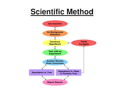 |
| map for science? |
You were probably told sometime early on about the map for science: the scientific method. It was probably displayed for your high school class as a tidy flowchart showing how a hypothetico-deductive approach allows scientists to solve problems. Scientists make observations about the natural world, gather data, and come up with a possible explanation or hypothesis. They then deduce the predictions that follow, and design experiments to test those predictions. If you falsify the predictions you then circle back and refine, alter, or eventually reject the hypothesis. Scientific progress arises from this process. Sure, you might adjust your hypothesis a few times, but progress is direct and straightforward. Scientists aren’t shown getting lost.
Then, once you actively do research, you realize that formulation-reformulation process dominates. But because for most applications the formulation-reformulation process is slow – that is, each component takes time (e.g. weeks or months to redo experiments and analyses and work through reviews) – you only go through that loop a few times. So you usually still feel like you are making progress and moving forward.
But if you want to remind yourself just how twisting and meandering science actually is, spend some time fitting dynamic models. Thanks to Ben Bolker’s indispensible book, this also comes with a map, which shows how closely the process of model fitting mirrors the scientific method. The modeller has some question they wish to address, and experimental or observational data they hope to use to answer it. By fitting or selecting the best model for they data, they can obtain estimates for different parameters and so hopefully test predictions from they hypothesis. Or so one naively imagines.
 |
| From Bolker's Ecological Models and Data in R, a map for model selection. |
“Consider the number of different models that can be constructed from the simple Lotka-Volterra formulation of interactions between two species, layering on realistic complexities one by one. First, there are at least three qualitatively distinct kinds of interaction (competition, predation, mutualism). For each of these we can have either an implicit accounting of basal resources (as in the Lotka-Volterra model) or we can add an explicit accounting in one particular way. That gives six different models so far. We can then add spatial heterogeneity or not (x2), temporal heterogeneity or not (x2), stochasticity or not (x2), immigration or not (x2), at least three kinds of functional relationship between species (e.g., predator functional responses, x3), age/size structure or not (x2), a third species or not (x2), and three ways the new species interacts with one of the existing species (x3 for the models with a third species). Having barely scratched the surface of potentially important factors, we have 2304 different models. Many of them would likely yield the same predictions, but after consolidation I suspect there still might be hundreds that differ in ecologically important ways.”Model fitting/selection, can actually be (speaking for myself, at least) repetitive and frustrating and filled with wrong turns and dead ends. And because you can make so many loops between formulation and reformulation, and the time penalty is relatively low, you experience just how many possible paths forward there to be explored. It’s easy to get lost and forget which models you’ve already looked at, and keeping detailed notes/logs/version control is fundamental. And since time and money aren’t (as) limiting, it is hard to know/decide when to stop - no model is perfect. When it’s possible to so fully explore the path from question to data, you get to suffer through realizing just how complicated and uncertain that path actually is.
 |
| What model fitting feels like? |
Bolker hints at this (but without the angst):
“modeling is an iterative process. You may have answered your questions with a single pass through steps 1–5, but it is far more likely that estimating parameters and confidence limits will force you to redefine your models (changing their form or complexity or the ecological covariates they take into account) or even to redefine your original ecological questions.”
I bet there are other processes that have similar aspects of endless, frustrating ability to consider every possible connection between question and data (building a phylogenetic tree, designing a simulation?). And I think that is what science is like on a large temporal and spatial scale too. For any question or hypothesis, there are multiple labs contributing bits and pieces and manipulating slightly different combinations of variables, and pushing and pulling the direction of science back and forth, trying to find a path forward.
(As you may have guessed, I spent far too much time this summer fitting models…)
(As you may have guessed, I spent far too much time this summer fitting models…)
Friday, August 21, 2015
#ESA100: The next dimension in functional ecology
The
third day of ESA talks saw an interesting session on functional ecology
(Functional Traits in Ecological Research: What Have We Learned and Where Are
We Going?), organized by Matt Aiello-Lammens and John Silander Jr.
As outlined by McGill and colleagues
(2006), a functional trait-based approach can help us move past idiosyncrasies
of species to understand more general patterns of species interactions and
environmental tolerances. Despite our common conceptual framework that traits
influence fitness in a given environment, many functional ecology studies have
been challenged to explain much variation in measured functional traits using
underlying environmental gradients. We might attribute this to a) measuring the
‘wrong’ traits or gradients, b) several trait values or syndromes being equally
advantageous in a given environment, or c) limitations in our statistical
approaches. Several talks in this organized session built up a nuanced story of
functional trait diversity in the Cape Floristic Region (CFR) of South Africa.
Communities are characterized by high species but low functional turnover (Matt
Aiello-Lammens; Jasper
Slingsby), and only in some genera do we see strong relationships between trait
values and environments (Matt Aiello-Lammens; Nora Mitchell). Nora Mitchell presented a novel Bayesian
approach combining trait and environmental information that allowed her to
detect trait-environment relationships in about half of the lineages she
investigated. These types of approaches that allow us to incorporate
phylogenetic relationships and uncertainty may be a useful next step in our
quest to understand how environmental conditions may drive trait patterns.
Another ongoing challenge in functional
ecology is the mapping of function to traits. This is complicated by the fact
that a trait may influence fitness in one environment but not others, and by
our common use of ‘soft’ traits, which are more easily measurable correlates of
the trait we really think is important. Focusing on a single important drought
response trait axis in the same CFR system described above, Kerri Mocko
demonstrated that clades of Pelargonium exhibited two contrasting
stomatal behaviours under dry conditions: the tendency to favor water balance
over carbon dioxide intake (isohydry) and the reverse (anisohydry). More to my
point, she was able to link a more commonly measured functional trait (stomatal
density) to this drought response behavior.
Turning from the macroevolutionary to
the community scale, Ben Weinstein evaluated the classic assumption of trait-matching
between consumer (hummingbird beak length) and resource (floral corolla length),
exploring how resource availability might shape this relationship. Robert
Muscarella then took a community approach to understanding species
distributions, testing the idea that we are most likely to find species where
their traits match the community average (community weighted mean). He used
three traits of woody species to do so, and perhaps what I found most
interesting about this approach was his comparison of these traits – if a
species is unlike the community average along one trait dimension, are they
also dissimilar along the other trait dimensions?
Thinking of trait dimensions, it was
fascinating to see several researchers independently touch on this topic. For
my talk, I subsampled different numbers and types of traits from a monkeyflower
trait dataset to suggest that considering more traits may be our best sampling
approach, if we want to understand community processes in complex,
multi-faceted environments. Taking trait dimensionality to the extreme, perhaps
gene expression patterns can be used to shed light on several important
pathways, potentially helping us understand how plants interact with their
environments across space and time (Andrew Latimer).
To me, this session highlighted
several interesting advances in functional ecology research, and ended with an
important ‘big picture’. In the face of another mass extinction, how is
biodiversity loss impacting functional diversity (Matthew Davis)?
McGill, B. J., Enquist, B. J., Weiher, E., & Westoby, M.
(2006). Rebuilding community ecology from functional traits. Trends in
ecology & evolution, 21(4), 178-185.
Thursday, August 13, 2015
#ESA100 The big-data era: ecological advances through data availability
Ecology is in a time of transition –from small-scale studies
being the norm to large, global datasets employed to test broad generalities. Along
with this ‘big data’ trend is the change in the ethical responsibility of
scientists who receive public funds to share their data and ensure public
access. As a result big online data repositories have been popping up
everywhere.
One thing that I have been doing while listening to talks, or
talking with people, is to make note of the use of large online databases. It
is clear that the use of these types of data has become commonplace. So much
so, that in a number of talks, the speakers simply referred to them by acronyms
and we all understood what it was that they used. Here are examples of online
data sources I heard referenced (and there are certainly many more):
Despite the attractiveness of huge amounts of data available online, such data can only paint broad pictures of patterns in nature and cannot capture small scale variability very well (Simberloff 2006). We still require detailed experiments and trait measurements at small scales for things like within-species trait variability.
Ecology has grown, and will continue to do so as data is made available. Yet, the classic ecological field experiment will continue to be the mainstay for ecological advancement into the future.
Simberloff, D. (2006) Rejoinder to Simberloff (2006): don't calculate effect sizes; study ecological effects. Ecology Letters, 9, 921-922.
Wednesday, August 12, 2015
#ESA100 Have system -need science! The opportunities for green roof ecology
 |
| Chicago City Hall green roof, adapted from Wikipedia (CC-BY-SA 3.0) |
I would argue strongly that urban systems, like green roofs,
are understudied and that these systems are the very places that ecological
concepts and theories can have relevance. My medical colleagues study human
physiology or microbiology in order to cure sick people –their science has
direct application to improving the world and human well being, and ecologists
have the same opportunity. Like a sick patient, urban systems are where our
science can have the greatest impact and can provide the most benefit. Urban
systems are under direct management and provide ample opportunity to manipulate
ecological patterns and processes in order to test theory and manage societal
benefits.
Time to study cities!
Tuesday, August 11, 2015
#ESA100 Declining mysticism: predicting restoration outcomes.
Habitat restoration literature is full of cases where the
outcomes of restoration activities are unpredictable, or where multiple sites
diverge from one another despite identical initial restoration activities. This
apparent unpredictability in restoration outcomes is often attributed to
undetected variation in site conditions or history, and thus have a mystical
quality where the true factors affecting restoration are just beyond our
intellect. These types of idiosyncrasies have led some to question whether
restoration ecology can be a predictable science.
 |
| Photo credit: S. Yasui |
The oral session “Toward prediction in the restoration of
biodiversity”, organized by Lars Brudvig, showed how restoration ecologists are
changing our understanding of restoration, and shedding light on the mystical
qualities of success. What is clear from the assembly of great researchers and
fascinating talks in this session is that recent ecological theories and
conceptual developments are making their way into restoration. Each of the 8 of
10 talks I saw (I had to miss the last two) added a novel take on how we
predict and measure success, and the factors that influence it. From the
incorporation of phylogenetic diversity to assess success (Becky Barak) to measuring dispersal
and establishment limitation (Nash Turley), and from priority effects (Katie
Stuble) to plant-soil feedbacks (Jonathan Bauer), it is clear that predicting
success is a multifaceted problem. Further, from Jeffry Matthews talk on
trajectories, even idiosyncratic restoration trajectories can be grouped into
types of trajectories (e.g., increasing diversity vs plateauing) and then
relevant factors can be determined.
What was most impressive about this session was the
inclusion of coexistence theory and basic demography into understanding how
species perform in restoration. Two talks in particular, one from Loralee
Larios on coexistence theory and the other from Dan Laughlin on predicting
fitness from traits by environment interactions, shed new light on predicting
restoration. Both of these talks showed how species traits and local
environmental conditions influence species’ demographic responses and the
outcome of competition. These two talks revealed how basic ecological theory
can be applied to restoration, but more importantly, and perhaps under-appreciated,
these talks show how our basic assumptions about traits and interactions with
other species and the environment require ground-truthing to be applicable to important
applied problems.
Subscribe to:
Posts (Atom)