print(santatraits)
                       heft transport first.appearance
Coca.cola.Santa         fat  reindeer             1900
Department.Store.Santa  fat  reindeer             1900
Salvation.Army.Santa    fat  reindeer             1890
Kriss.Kringle           fat  reindeer             1800
Santa.Claus             fat  reindeer             1700
Pere.Noel              thin    donkey             1400
Father.Christmas        fat      foot             1400
Sinterklaas            thin     horse              400
Saint.Nicholas         thin      foot              300
Ded.Moroz              thin      foot             1937
We are fortunate to also have sequence data (from DNA on milk glasses and lost beard hairs), so we can add additional information about relatedness amongst these species.
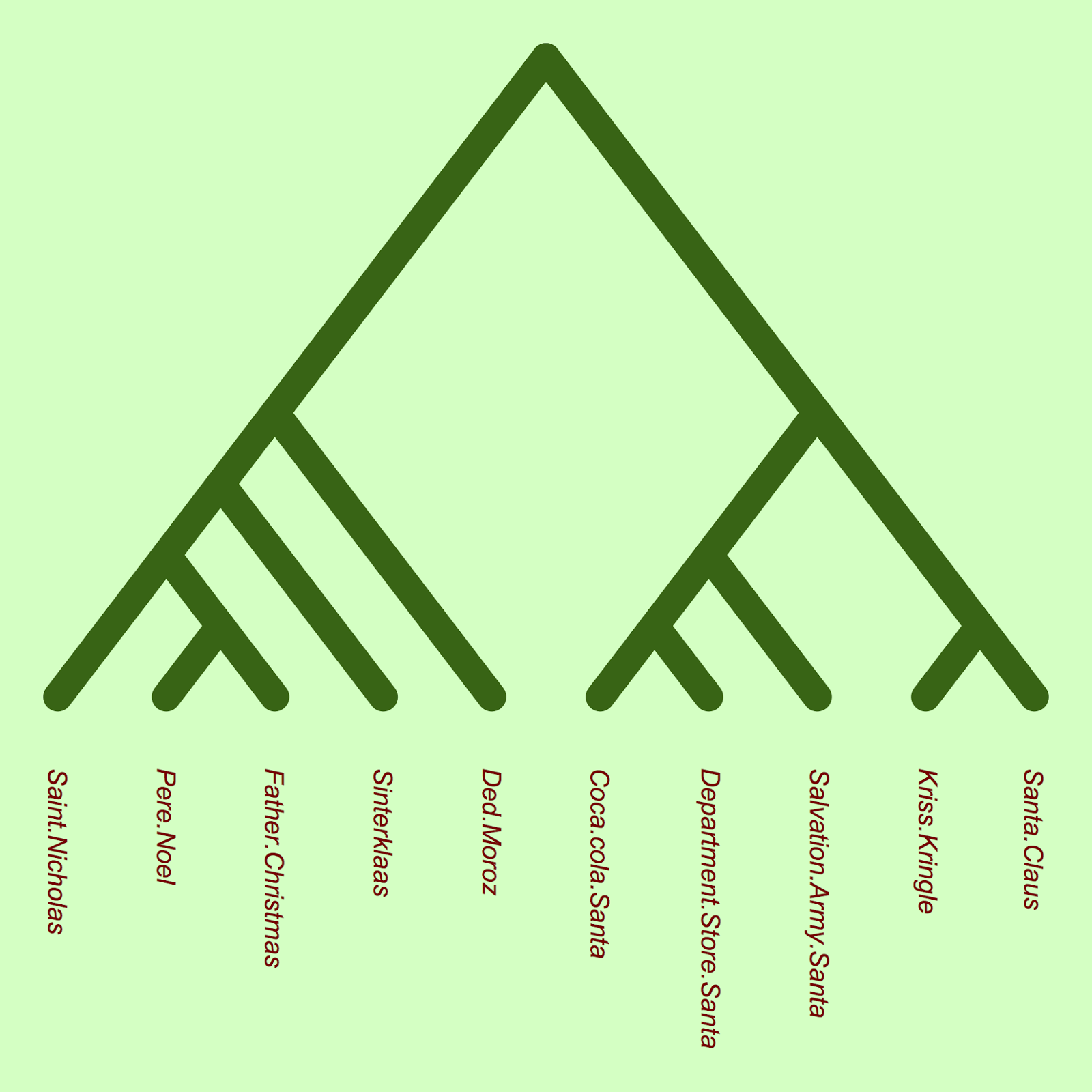
plot(xmas.tree, type = "c", FALSE, edge.color="darkgreen", edge.lty=1, edge.width=18, label.offset = 1, direction="downward", font=3, tip.color="darkred")

The phylogeny shows that there seems to be an early divergence between European and North American santas. Indeed, there is a group of North American santas (Mall Santa, Coca-cola Santa, Salvation Army Santa) which are closely related (and also appear to share very similar traits, based on the table above). (Note that branch lengths in this phylogeny show nucleotide substitutions, and it is not time-calibrated, due to the absence of santa fossils).
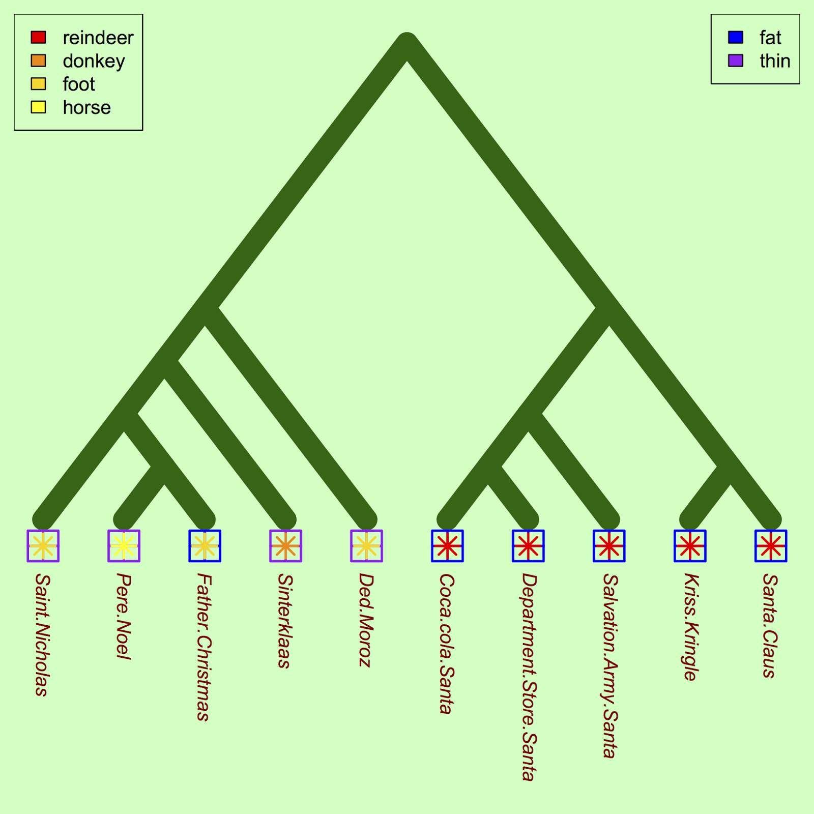
One approach is to identify a few traits and plot them on the phylogeny to compare how traits vary among santas. Let's start with anatomical characteristics:
#Plot traits (fatness) against Santa
co1 = c("blue", "purple")
tiplabels(pch = 12, col = co1[as.factor(heft)], cex = 3.5, adj=c(0.5, 0), lwd=2)

#Let's see the transportation mode trait too:
co2 <- c("yellow", "gold", "darkorange", "red")
tiplabels(pch = 8, col = co2[as.factor(transport)], cex = 2, adj=c(0.5, 0), lwd=2)

#Legends
legend("topleft", legend=c("reindeer", "donkey", "foot", "horse"), fill=rev(c("yellow", "gold", "darkorange", "red")))
legend("topright", legend=c("fat", "thin"), fill=c("blue", "purple"))

For a future study, we could ask whether the apparent correlation between fatness and reindeer usage is significant, once the underlying phylogenetic relationships were controlled for.
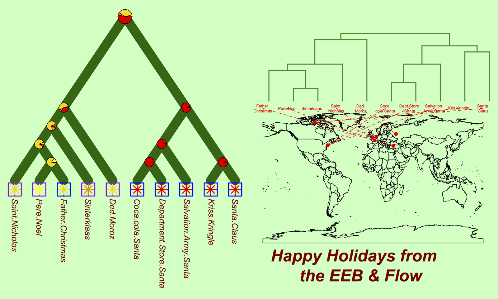
We can also reconstruct santa traits (here, we look at the form of transportation) to explore what form of transportation ancestral santas likely used:
#reconstruct ancestral state
cc = ace(transport, xmas.tree, type="discrete")
co2 = c("yellow", "gold", "darkorange", "red")
nodelabels(pie = cc$lik.anc, piecol = co2, cex = c(1.5, rep(1, 8)))
The markers at each node show the probability that this ancestral taxa used each of the four possible types of transportation. It seems that the North American santas and their ancestors have long relied on a trusty reindeer mutualism.
Finally, we can look at the geography of all the various santas:
phylo.to.map(xmas.tree, locales)

To run this caRd yourself, follow the link to the R code: https://gist.github.com/cmtucker/8e5677bdd5c409d70738


3 comments:
Wow, great and impressive analysis! However there's a little glitch in the primary data: Sinterklaas uses a white horse (named "amerigo") and a steamboat for short and long distance transportation, respectively.
Clearly the data is incomplete! Apologies, I'm afraid Wikipedia was my primary research tool (shame!).
Reindeer alternatives: http://birdandmoon.com/comic/reindeer-alternatives/
Post a Comment