I had a busy year, and it completely slipped my mind that I usually do a caRd for the blog! So it's a little late, but hopefully provides a little end of year cheeR ;-)
A short warning: I've stopped trying to make these compatible with RStudio. I know that RStudio is very popular, but I struggle to get its internal plotting device to update iteratively to make an animation (despite trying various things, like while() or if() statements, or Sys.sleep()). If someone has a solution, please share.
To enjoy these plots you should see the animation in real time: e.g. Base R (any operating system) or R run via emacs or vim.
To run, you can access the source file on github
or run this code:
source("https://tinyurl.com/2018rcard")
If you prefer not to run the code, the gif version can be found here!
Showing posts with label R. Show all posts
Showing posts with label R. Show all posts
Thursday, December 27, 2018
Monday, December 18, 2017
Holiday caRd 2017!
Here is this year's card, with best wishes from both of us at the EEB & Flow!
It gets a little harder every year to figure these out. R's plotting capabilities improve every year, but usually via specialized packages. I've tried more and more to use as few additional packages beyond base, and to produce a script that is hopefully compatible across platforms.
OR, the easiest way, run this quick code directly:
Full script here.
(Bonus points for those who can guess which species of McArthur's warblers these are meant to be ;) )
- For best performance, users must install the 'deldir' package and the 'RCurl' package. This lets you download the necessary data file with as little effort as possible.
- If you have trouble accessing the file via the URL, you can just download the data file from Github directly, making sure to load the file into R using the hashed out code in Lines6-7.
OR, the easiest way, run this quick code directly:
Full script here.
(Bonus points for those who can guess which species of McArthur's warblers these are meant to be ;) )
Monday, December 19, 2016
2016 holiday caRd
Once more, tis the season! Hope you had an excellent year of science and R coding. This card requires the igraph library - it (loosely) relies on an infection (S-I model) moving through a network :-)
To view season's greetings from 2016:
Go to the gist and download the file directly ("download gist") or hit "raw" and copy/paste. Or, copy and paste the code below.
Users of Rstudio will not be able to see the animation, so base R is highly recommended.
For those not able or willing to run the card, you can view it and the past years' cards here!
Tuesday, December 15, 2015
2015 caRd - A diveRsity of Santas
A keen observer will note that there are a number of similar taxa that are active this time of year.
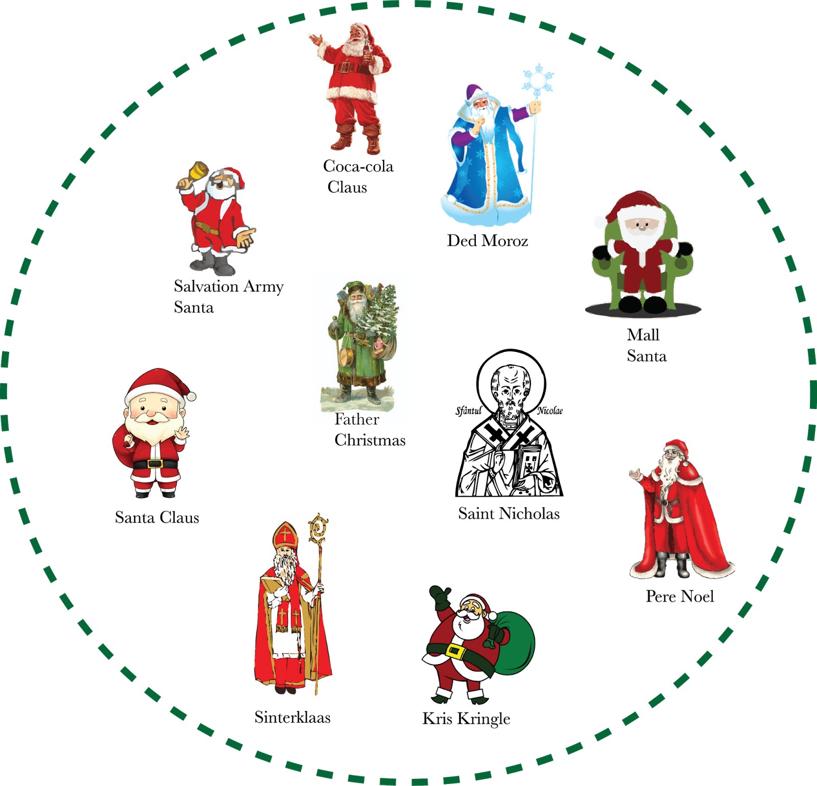
Although well described in the literature, surprisingly little attention has been given to the ecology of these creatures. Observational data allows some traits to be compiled, however, and some simple exploratory analyses may allow us to better understand the 'Santa' assemblage.
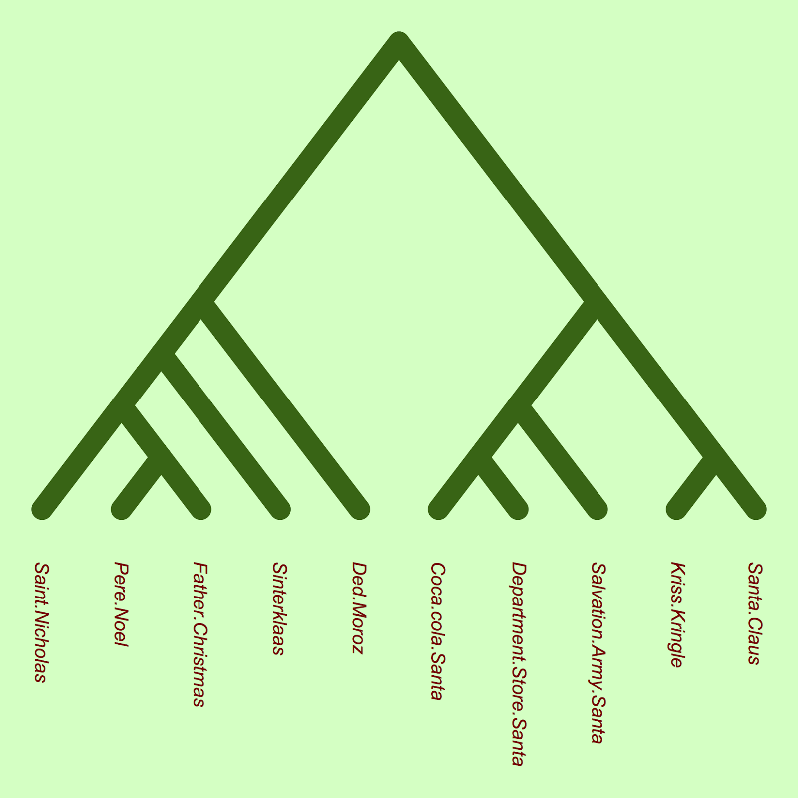
We are fortunate to also have sequence data (from DNA on milk glasses and lost beard hairs), so we can add additional information about relatedness amongst these species.
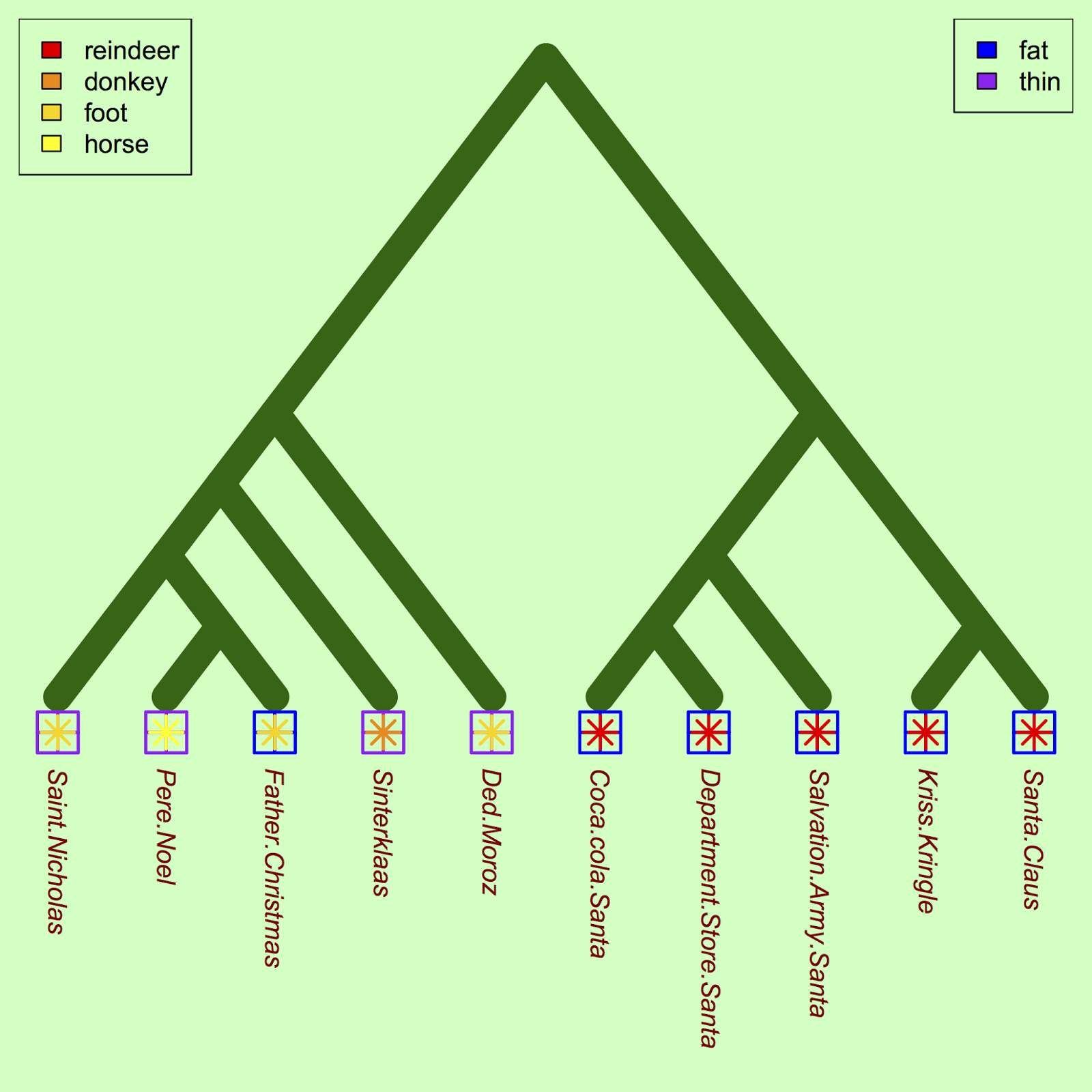
One approach is to identify a few traits and plot them on the phylogeny to compare how traits vary among santas. Let's start with anatomical characteristics:
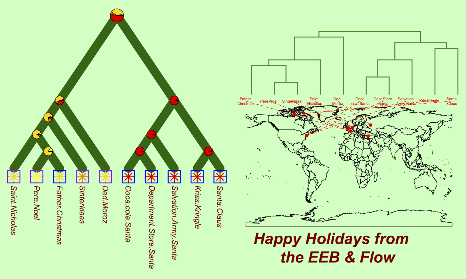
Finally, we can look at the geography of all the various santas:

print(santatraits)
                       heft transport first.appearance
Coca.cola.Santa         fat  reindeer             1900
Department.Store.Santa  fat  reindeer             1900
Salvation.Army.Santa    fat  reindeer             1890
Kriss.Kringle           fat  reindeer             1800
Santa.Claus             fat  reindeer             1700
Pere.Noel              thin    donkey             1400
Father.Christmas        fat      foot             1400
Sinterklaas            thin     horse              400
Saint.Nicholas         thin      foot              300
Ded.Moroz              thin      foot             1937
We are fortunate to also have sequence data (from DNA on milk glasses and lost beard hairs), so we can add additional information about relatedness amongst these species.
plot(xmas.tree, type = "c", FALSE, edge.color="darkgreen", edge.lty=1, edge.width=18, label.offset = 1, direction="downward", font=3, tip.color="darkred")

The phylogeny shows that there seems to be an early divergence between European and North American santas. Indeed, there is a group of North American santas (Mall Santa, Coca-cola Santa, Salvation Army Santa) which are closely related (and also appear to share very similar traits, based on the table above). (Note that branch lengths in this phylogeny show nucleotide substitutions, and it is not time-calibrated, due to the absence of santa fossils).
One approach is to identify a few traits and plot them on the phylogeny to compare how traits vary among santas. Let's start with anatomical characteristics:
#Plot traits (fatness) against Santa
co1 = c("blue", "purple")
tiplabels(pch = 12, col = co1[as.factor(heft)], cex = 3.5, adj=c(0.5, 0), lwd=2)

#Let's see the transportation mode trait too:
co2 <- c("yellow", "gold", "darkorange", "red")
tiplabels(pch = 8, col = co2[as.factor(transport)], cex = 2, adj=c(0.5, 0), lwd=2)

#Legends
legend("topleft", legend=c("reindeer", "donkey", "foot", "horse"), fill=rev(c("yellow", "gold", "darkorange", "red")))
legend("topright", legend=c("fat", "thin"), fill=c("blue", "purple"))

For a future study, we could ask whether the apparent correlation between fatness and reindeer usage is significant, once the underlying phylogenetic relationships were controlled for.
We can also reconstruct santa traits (here, we look at the form of transportation) to explore what form of transportation ancestral santas likely used:
#reconstruct ancestral state
cc = ace(transport, xmas.tree, type="discrete")
co2 = c("yellow", "gold", "darkorange", "red")
nodelabels(pie = cc$lik.anc, piecol = co2, cex = c(1.5, rep(1, 8)))
The markers at each node show the probability that this ancestral taxa used each of the four possible types of transportation. It seems that the North American santas and their ancestors have long relied on a trusty reindeer mutualism.
Finally, we can look at the geography of all the various santas:
phylo.to.map(xmas.tree, locales)

To run this caRd yourself, follow the link to the R code: https://gist.github.com/cmtucker/8e5677bdd5c409d70738
Monday, December 15, 2014
Holiday caRd 2014: Snowflakes
Apparently it's that time of year again! The R circlize package plays a prominent role in this caRd.
Like snowflakes, no two cards are likely to be identical, so try it a few times :)
Lots of options for viewing the R code:
1) Run it automatically by just using the following few lines of R code. Probably the easiest way, provided you've installed RCurl: it allows you to directly run the github code from its url.
install.packages("RCurl")
2) Go to https://gist.github.com/cmtucker/c591e868c76de1ac81e6 and access directly. You can download the file directly ("download gist") or hit "raw" and copy/paste.
3) Copy and paste the code below.
library(RCurl)
options(RCurlOptions = list(verbose = FALSE, capath = system.file("CurlSSL", "cacert.pem", package = "RCurl"), ssl.verifypeer = FALSE))
#this seems necessary for the Windows people only?
#
eval(expr = parse(text = getURL("https://gist.githubusercontent.com/cmtucker/c591e868c76de1ac81e6/raw/ea3581a2d7f10810023529c7046edb40f099cbb3/snowflakeCode")))
2) Go to https://gist.github.com/cmtucker/c591e868c76de1ac81e6 and access directly. You can download the file directly ("download gist") or hit "raw" and copy/paste.
3) Copy and paste the code below.
Tuesday, December 17, 2013
Holiday caRd 2013
A holiday pResent made of competition from the EEB & Flow :-)
(Easy to copy and run if you choose "view raw" in the lower right hand corner. Just copy and paste into R, it will do all the work. You will need to download and install R if you don't already have it.)
(Easy to copy and run if you choose "view raw" in the lower right hand corner. Just copy and paste into R, it will do all the work. You will need to download and install R if you don't already have it.)
Wednesday, December 12, 2012
holiday caRd from the EEB & Flow 2012
To celebrate the start of the holiday season for many of us, the end of exams and marking for others, and for fellow Canadians, snow, enjoy this caRd from the EEB & flow! We will see you around the New Year with our traditional year-end post about the current state of ecology.
Or, copy and paste the code here into your R console.
Sunday, December 18, 2011
holiday caRd
I wasn't planning on making any more "caRds", but since I received a number of requests, find below a holiday card from the EEB & flow. For optimal viewing, perhaps throw some Jingle Bells on in the background.
###holiday caRd
#install "rgl" package if necessary:
install.packages("rgl")
This code relies heavily on the rgl package in R. Be sure to run the first line of code to install this package if you don't already have it.
###holiday caRd
#install "rgl" package if necessary:
install.packages("rgl")
#load library
library(rgl)
##Data
r=1.0
h=5.0
m=h/r
x=seq(0:99)
y=x
X=x*cos(y)
Y=x*sin(y)
Z=-1*(m*x)
Z1=Z+rnorm(length(Z),Z,5)
sub<-matrix(subset(c(X,Y,Z),Z==max(Z)),ncol=3)
trunk<-matrix(c(0.54,0.84,-200,0.54,0.84,-650),byrow=TRUE,ncol=3)
sno<-c(0,rep(15,9))
##Plot card
open3d(FOV=1)
par3d(windowRect=c(100,100,600,600))
bg3d("aquamarine2")
plot3d(X,Y,Z,col="darkgreen",type="l",box=FALSE,axes=FALSE,lwd=10,zlim=c(min(Z),0),xlab="",ylab="",zlab="",top=TRUE,border=TRUE)
plot3d(X,Y,Z,col=c("yellow","red"),add=TRUE,type="s",radius=3)
points3d(sub,col="orange",size=10)
lines3d(trunk,col="brown",lwd=20)
text3d(matrix(c(0.54,-100,300),ncol=3),text="Happy Holidays",font=5,cex=1.9,color="darkred",adj=c(0.5,1))
text3d(matrix(c(0.54,0.84,-650),ncol=3),text="and",font=5,cex=1.5,color="darkred",adj=c(0.5,1))
text3d(matrix(c(0.54,75,-780),ncol=3),text="a Happy New Year",font=5,cex=1.9,color="darkred",adj=c(0.5,1))
mat<-par3d("scale")
##Play card
for(i in 1:10){
par3d(scale=mat,ignoreExtent=TRUE)
points3d(matrix(c(sample(-160:160,sno[i]),sample(-160:160,sno[i]),sample(-500:150,sno[i])),ncol=3),col="white",size=3)
play3d(spin3d(axis=c(0,0,1)),duration=1)
if(i==10){points3d(sub,col="darkorange",size=17)
plot3d(X,Y,Z,col=c("yellow","red"),type="s",radius=4,add=TRUE) } }
text3d(matrix(c(0,140,-900),ncol=3),text="From the EEB & Flow",font=1,cex=1.0,color="darkgreen",adj=c(0.5,1))
##The rgl device window allows you to use your mouse to manipulate the plot in 3-dimensions, so feel free to do so before closing it.
You can also access the script here.
Thursday, October 27, 2011
halloween caRd
To view the card, run the code below using R
###########################################################################
###required libraries
##if you do not have the "fields" and "MBA" libraries, you need this step to install them
install.packages("fields")
install.packages("MBA")
## load libraries
library(fields)
library(MBA)
###data
data<-matrix(c(44.9186,81.0824,46.9512,80.1061,49.187,80.7055,57.9268,80.1493,60.3659,81.34,69.3089,80.1941,78.4553,79.2459,91.8699,70.834,99.7967,55.9047,101.2195,30.9102,96.1381,17.3075,85.5691,7.4235,74.3902,4.2299,61.7886,1.8181,55.4878,1.0059,49.187,0.9811,45.3252,1.7532,37.1951,1.9181,20.3252,7.1666,8.9431,17.1612,4.2683,29.1507,4.2683,50.8042,9.5528,66.3761,18.4959,76.2539,29.065,80.6261,38.6179,80.8607,44.9186,81.0824),ncol=2,byrow=TRUE)
stem<-matrix(c(60.3659,81.34,57.9268,80.1493,49.187,80.7055,46.9512,80.1061,44.9186,81.0824,45.5285,83.6438,47.561,88.1794,44.1057,97.2209,48.7805,99.9952,54.878,87.6176,60.3659,81.34),ncol=2,byrow=TRUE)
eye<-matrix(c(45.935,46.4407,34.1463,44.8195,36.7886,46.9952,36.382,50.9306,32.3171,53.08,29.065,53.0672,26.0163,49.7086,28.0488,45.1892,20.3252,48.7021,20.1219,55.3942,23.5772,61.1164,30.8942,65.476,32.3171,59.7729,45.935,46.4407),ncol=2,byrow=TRUE)
eye2<-matrix(c(58.9431,46.6888,65.4472,51.2419,71.748,56.9754,74.3902,65.4504,82.7236,59.7745,84.9593,56.4368,84.7561,48.562,77.439,45.7772,78.8618,50.5072,74.3902,53.6393,69.9186,51.6532,68.6992,47.9083,70.5285,44.9627,58.9431,46.6888),ncol=2,byrow=TRUE)
mouth<-matrix(c(8.9431,44.7202,23.374,41.2338,30.0813,22.7562,38.2114,38.5363,65.0407,38.445,73.374,22.533,80.2846,40.8673,96.9512,44.673,93.4959,31.8641,84.1463,18.8352,66.2602,9.7097,61.9919,16.1889,59.3496,8.3045,45.5285,8.447,42.8862,16.1137,38.2114,9.4024,22.7642,17.4125,11.9919,31.7401,8.9431,44.7202),ncol=2,byrow=TRUE)
stars<-matrix(c(sample(seq(0,100),80),sample(seq(20,100),80,replace=TRUE)),ncol=2)
###plot
par(bg = "black")
par(mar=c(5,2,4,2))+0.1
plot(data,type="n",xlim=c(0,100),ylim=c(0,100),xaxt="n",yaxt="n",xlab="",ylab="",axes=FALSE)
symbols(x=stars[,1],y=stars[,2],circles=rep(0.001,nrow(stars)),inches=0.015,bg="white",xlim=c(0,100),ylim=c(0,100))
col<-runif(nrow(data),min=4,max=7)
datmb<-mba.surf(matrix(cbind(data,col),ncol=3),no.X=200,no.Y=200,extend=FALSE)
image(datmb$xyz,zlim=c(0,10),col=heat.colors(40),add=TRUE)
polygon(stem,col="darkgreen")
polygon(eye,col="yellow")
polygon(eye2,col="yellow")
polygon(mouth,col="yellow")
points(data,type="l")
mtext("Happy Halloween",side=3,col="green3",cex=3.5,font=4)
mtext("from the EEB and Flow",side=1,col="green3",cex=2.5,font=4)
Tuesday, May 11, 2010
Picante's coming out party
This past decade has seen a rapid expansion of the use of evolutionary phylogenies in ecological studies. This expansion is largely due to the increased availability of phylogenies, but has resulted in new types of hypotheses and statistics aimed to test the phylogenetic patterns underpinning ecological communities. The main computational tool used has been phylocom, created by Cam Webb, David Ackerly and Steve Kembel, which has its own binaries to be installed on one’s computer. However, a new R package, picante has been created by Steve Kembel and colleagues which runs many of the same routines as in phylocom, but in the R framework, allowing one to tie these analyses in better with other, non-phylogenetic tests. Picante also has a number of features and tests not found in phylocom, including tests of phylobetadiversity and phylogenetic signal using Blomberg’s K.
Thanks Steve for all your hard work and for making these tests available to everyone.
Kembel, S., Cowan, P., Helmus, M., Cornwell, W., Morlon, H., Ackerly, D., Blomberg, S., & Webb, C. (2010). Picante: R tools for integrating phylogenies and ecology Bioinformatics DOI: 10.1093/bioinformatics/btq166
Thanks Steve for all your hard work and for making these tests available to everyone.
Kembel, S., Cowan, P., Helmus, M., Cornwell, W., Morlon, H., Ackerly, D., Blomberg, S., & Webb, C. (2010). Picante: R tools for integrating phylogenies and ecology Bioinformatics DOI: 10.1093/bioinformatics/btq166
Monday, March 16, 2009
A roadmap to generalized linear mixed models
 In a recent paper in TREE, Ben Bolker (from the University of Florida) and colleagues describe the use of generalized linear mixed models for ecology and evolution. GLMMs are used more and more in evolution and ecology given how powerful they are, basically because they allow the use of random and fix effects and can analyze non-normal data better than other models. The authors made a really good job at explaining what to use when. Despite the fact that you need more than basic knowledge of stats to fully understand this guide, I think that people should take a look at it before starting to plan their projects, since it outlines really well all the possible alternatives (and challenges) that one can have when analyzing data. This article also describes what is available in each software package; this is really useful since is not obvious with program in SAS or R you need to use when dealing with some specific GLMMs.
Bolker, B., Brooks, M., Clark, C., Geange, S., Poulsen, J., Stevens, M., & White, J. (2009). Generalized linear mixed models: a practical guide for ecology and evolution Trends in Ecology & Evolution, 24 (3), 127-135 DOI: 10.1016/j.tree.2008.10.008
Sunday, February 8, 2009
Shortening the R curve
 I am a strong proponent of R for all data management, analysis and visualization. It is a truly egalitarian analysis package -open source and community-contributed analysis packages. The true power comes from complete control and automization of your analyzes as well as publicly accessible new functions created by members of the community. However, the drawback for a lot of people has been the rather steep learning curve, as with any programing language. But there are now a plethora of good books available that help shorten this curve. The Human Landscapes blog as reviewed and ranked introductory and reference R books, which should serve as an invaluable resource for those striving to become aRgonauts.
Subscribe to:
Posts (Atom)

